Introuction to Statistical Learning with Application in Python (Gareth James et al., 2023, 1st edition)
My answers to the exercices on ISLP
Answers
Books
Author
Natnael Getahun
Published
February 21, 2026
2.4 Exercises
Conceptual
1.
More flexible will be better.
Justification: as the number of data increases, we can be less concerned about variance, since new data points wouldn’t change the estimated f by that much. This means we can focus on decreasing bias, allowing us to focus on more flexible statistical learning methods.
Less flexible will be better.
Justification: With a large number of predictors and small umber of observations, new data points can change our estimated f by a lot, forcing us to be more careful about the effects of variance. We can’t afford flexibility as it will come with high variance, even if it decreases bias.
More flexible will be better.
Justification: With highly non-linear models, our concern lies that our estimated model will be far from the underlying model, i.e., huge bias. We can decrease bias by using more flexible methods.
Less flexible will be better.
Justification: with high variance of error terms, using highly flexible statistical learning methods risks following the noise rather than the patter in the data. Newer data points will have the ability to change the estimated f significantly. We can reduce this by using less flexible learning methods.
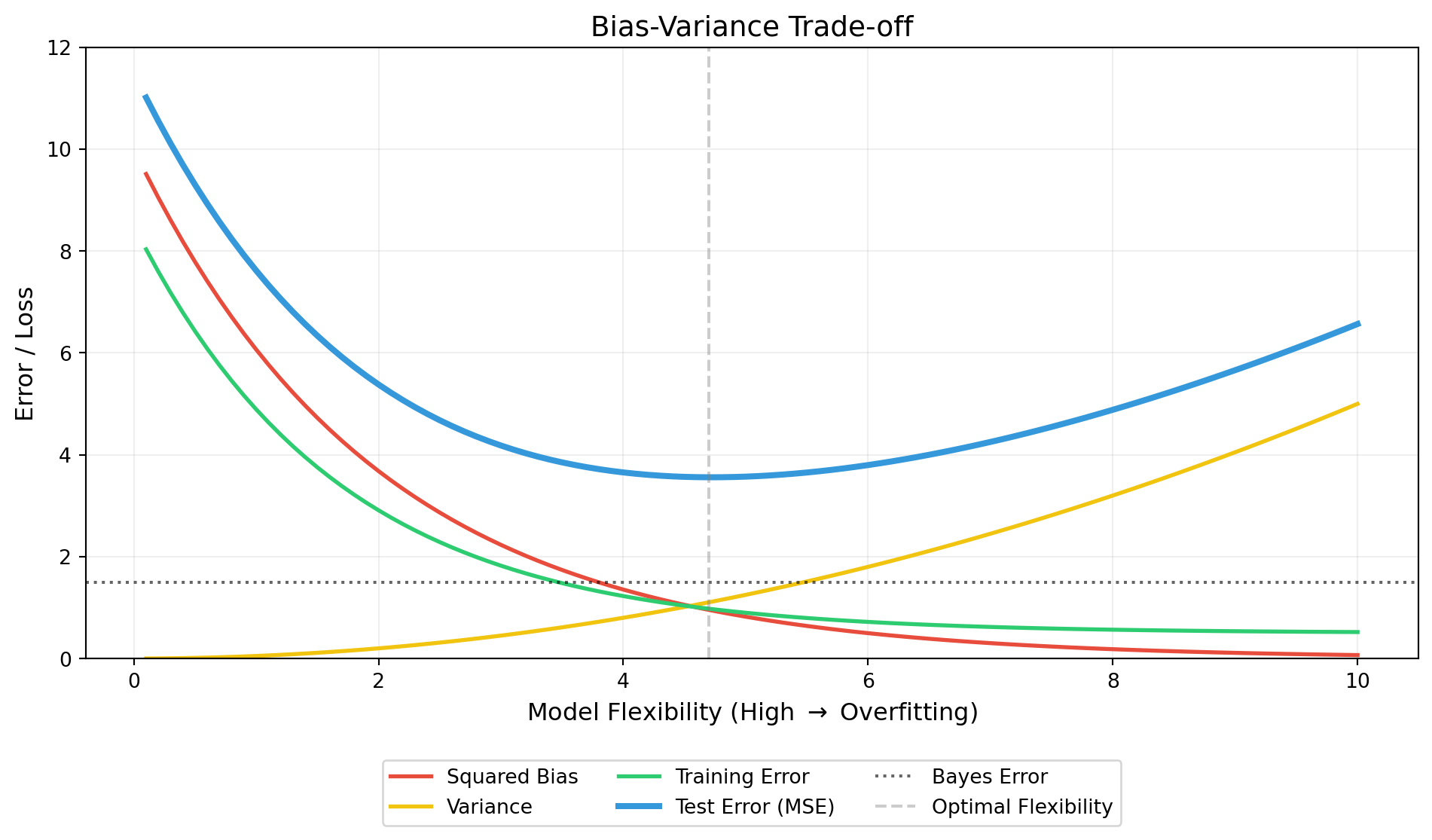
Squared bias: as the flexiblity increases, the estimated function has better chance to approximate the underlying function, reducing bias.
Variance: as flexibility increases, the functions starts mirroring the noise in the data rather than the underlying pattern. This makes sensitive to changes in data, increasing variance.
Bayes (irreducible) error: This is the limiting factor. It can be error caused as a result of unaccounted for predictors or an underlying, unexplainable noise. The test error cannot cross below this line.
Training error: as the flexibility increases, the statistical method better fits the training data, whether it will generalize well to the test set or not.
Test error: This is measures the accuracy of the model when tested on previously unseen data. It is the sum of the bayes error, variance, and squared bias. As flexibilty increases from none to its optimal value (where the sum of variance and square bias is at its lowest), the training error drops. After this optimal value however, more flexibility increases the variance significantly.
4.
Spam email detection, response = spam not spam, predictors = words and phrases used in the email, goal = prediction
Clustering based on attributes for better sampling
5.
Advantages: A very flexible approach can explain the data better when it is needed. Especially if relations are non-linear and rugged, a flexible approach can be useful. Flexible approaches result in models with lower bias.
Disadvantage: It can easily overfit the data, failing to generalize for unseen samples. I usually needs larger amounts of data than its less flexible alternatives when it works well.
A less flexible approach will be prefered in the case of fewer data. In cases were newly introduced data can change the model significantly.
6.
Parametric statistical learning approaches focus on finding parameters that can minimize certain loss functions (or maximize likelihood/ conditional probabilities of y given x). In other words, parameteric methods assume functional form. This approach makes parametric learning approaches simpler to build and easier to interpret. In cases where parameters are associated with predictors, we can infer and explain the effect of the predictors on the response variable. Non-parametric approaches don’t rely on finding values of parameters. This makes them harder to understand and difficult to interpret: they are primarily used for prediction purposes only, since inference is almost impossible.
def simple_knn(k=1): df = distance_df.sort_values(by='distance', ascending=True) df_of_interest = df.iloc[:k]return df_of_interest['Y'].mode().item()prediction = simple_knn() print(f'For K = 1 our prediction is: {prediction}')
For K = 1 our prediction is: Green
prediction = simple_knn(k=3)print(f'For K = 3 our prediction is: {prediction}')
For K = 3 our prediction is: Red
We need to choose ‘K’ so that KNN method becomes flexible enough to capture the non-linearity of the Bayes decision boundary. The lower or K the more flexible our methods becomes. We would expect the best value for K to be small.
Applied
8.
import pandas as pfcollege = pd.read_csv('data/College.csv')
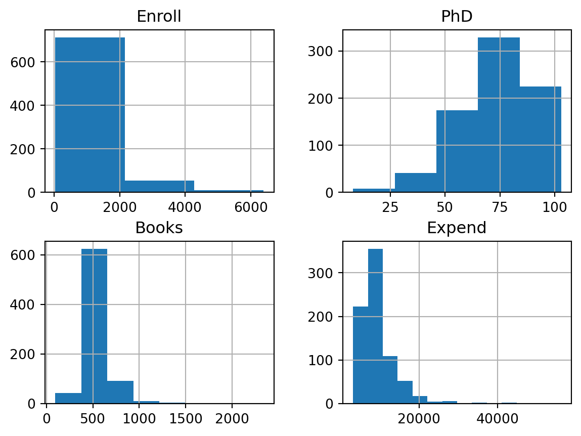
weight          350
name            304
mpg             129
acceleration     95
horsepower       94
displacement     82
year             13
cylinders         5
origin            3
dtype: int64
print('Name, year, cylinders, and origin can be seen as categorical values. \n"Year" however can be treated a discreet numerical data. \n"Horsepower" has its type misclassified.')
Name, year, cylinders, and origin can be seen as categorical values.
"Year" however can be treated a discreet numerical data.
"Horsepower" has its type misclassified.
for col in auto.columns:if'int'instr(auto[col].dtype) or'float'instr(auto[col].dtype):range= auto[col].max() - auto[col].min()print(col, '_range = ', range, sep='')
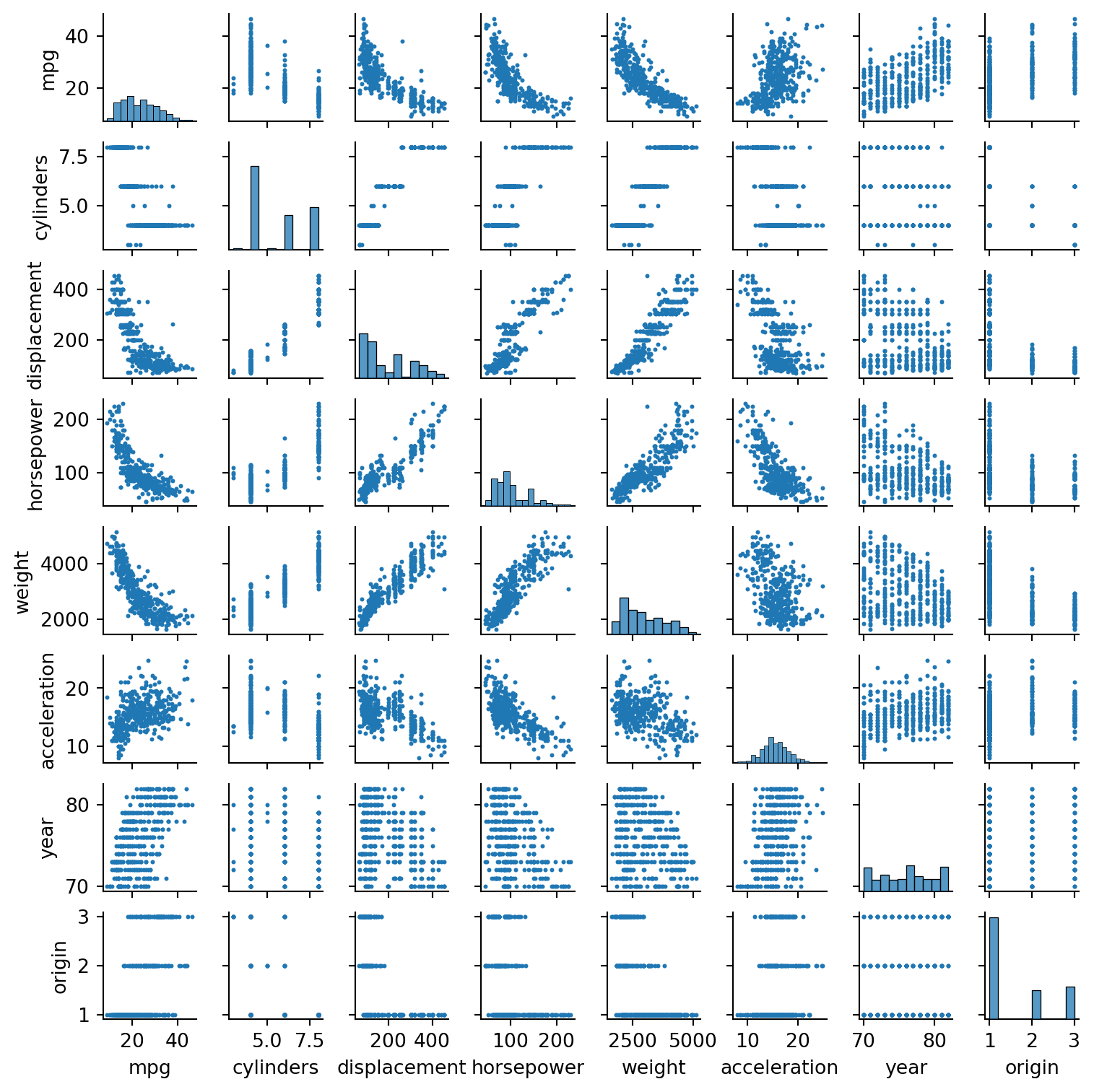
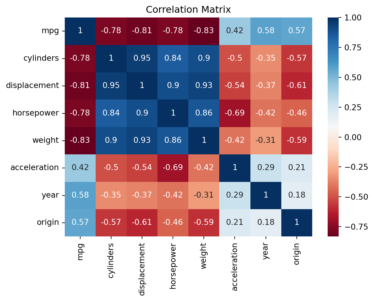
print('Notice while mpg is negatively correlated with most variables, a non-linear fit might better explain the data.\nIf we are using learning methods that make assumptions on the variance of the error term, we need to be careful about multicollinearity.')
Notice while mpg is negatively correlated with most variables, a non-linear fit might better explain the data.
If we are using learning methods that make assumptions on the variance of the error term, we need to be careful about multicollinearity.
print('We see strong correlations between "mpg" and other variables, whether postive or negative. \nWhile our correlation mapping suggests that a linear regression might do well, \nour scatter plots suggest we will benefit in exploring more flexible methods that can follow the slight non-linearity.')
We see strong correlations between "mpg" and other variables, whether postive or negative.
While our correlation mapping suggests that a linear regression might do well,
our scatter plots suggest we will benefit in exploring more flexible methods that can follow the slight non-linearity.
10.
from ISLP import load_databoston = load_data('Boston')boston.head()
crim
zn
indus
chas
nox
rm
age
dis
rad
tax
ptratio
lstat
medv
0
0.00632
18.0
2.31
0
0.538
6.575
65.2
4.0900
1
296
15.3
4.98
24.0
1
0.02731
0.0
7.07
0
0.469
6.421
78.9
4.9671
2
242
17.8
9.14
21.6
2
0.02729
0.0
7.07
0
0.469
7.185
61.1
4.9671
2
242
17.8
4.03
34.7
3
0.03237
0.0
2.18
0
0.458
6.998
45.8
6.0622
3
222
18.7
2.94
33.4
4
0.06905
0.0
2.18
0
0.458
7.147
54.2
6.0622
3
222
18.7
5.33
36.2
n_row = boston.shape[0]n_col = boston.shape[1]cols =''for col in boston.columns: cols += col +' 'print(f'There are {n_row} rows.')print(f'There are {n_col} cols.')print(f'The rows represent each instance/observation.\nThe columns represent the following variables: {cols}.')
There are 506 rows.
There are 13 cols.
The rows represent each instance/observation.
The columns represent the following variables: crim zn indus chas nox rm age dis rad tax ptratio lstat medv .
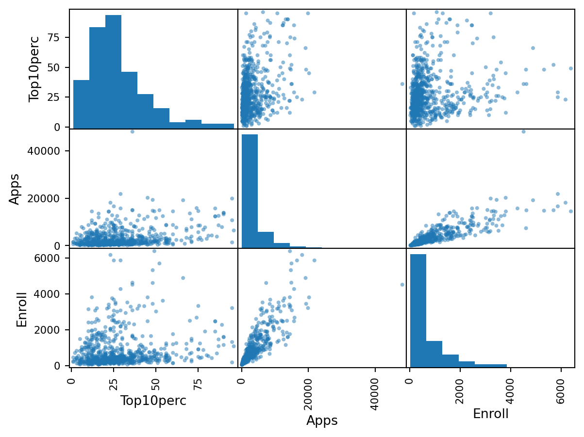
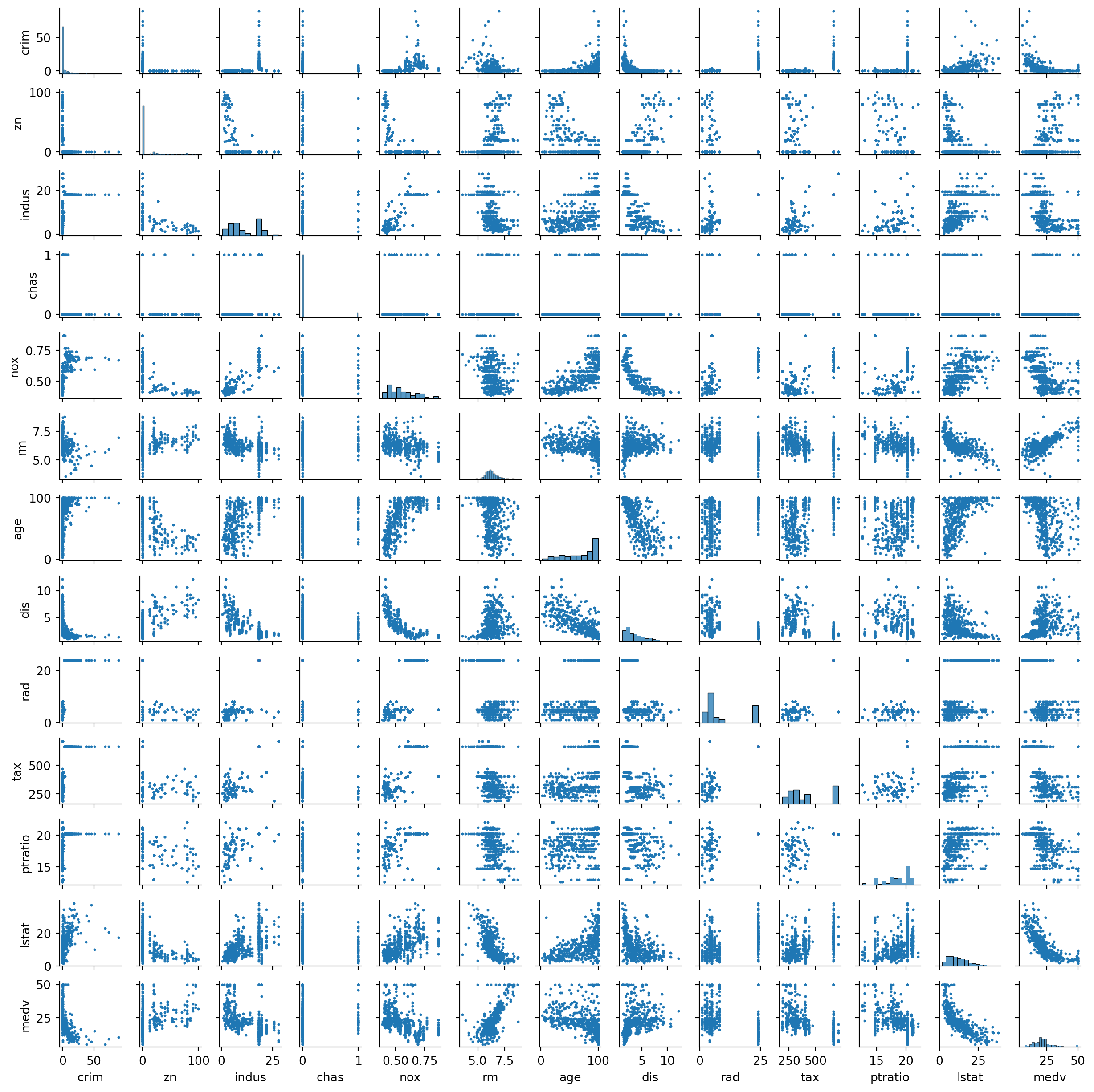
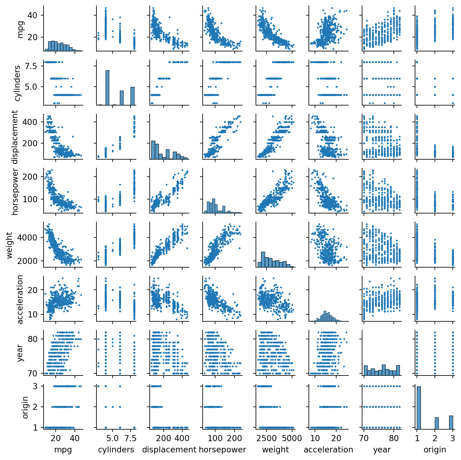
sns.pairplot(boston, height=1, plot_kws= {'linewidth':0, 's':5})print('We can suspect "rad", "tax", "ptratio" variables have been capped or had their missing values filled or have a strong "mode".\nTransformation of per capita crime rate can help out our model.\nTransformation of other variables as well might not be a bad idea.\nMight need to be careful with multicollinearity.')
We can suspect "rad", "tax", "ptratio" variables have been capped or had their missing values filled or have a strong "mode".
Transformation of per capita crime rate can help out our model.
Transformation of other variables as well might not be a bad idea.
Might need to be careful with multicollinearity.
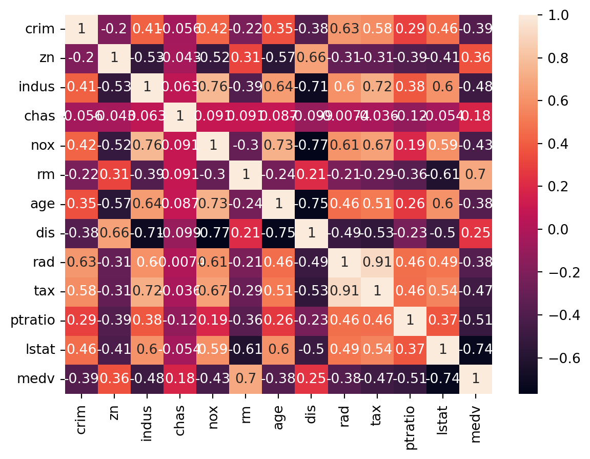
sns.heatmap(boston.corr(numeric_only=True), annot=True)print('Many variables promise to be associated with per cpaita crime rate. \n"nox", "age", and "lstat" appear to be positively correlated, \nwhile we should be creaful about claiming "rad" and "tax" as good predictors as the story person correlation and our scatter plots tell as are not the same.\n"medv", "dis", and "rm" appear to be negatively correlated with per capita crime rate.')
Many variables promise to be associated with per cpaita crime rate.
"nox", "age", and "lstat" appear to be positively correlated,
while we should be creaful about claiming "rad" and "tax" as good predictors as the story person correlation and our scatter plots tell as are not the same.
"medv", "dis", and "rm" appear to be negatively correlated with per capita crime rate.
for col in boston.columns:if'int'instr(boston[col].dtype) or'float'instr(boston[col].dtype):range= boston[col].max() - boston[col].min()print(col, '_range = ', range, sep='')
Intercept: \[\begin{aligned}
H_0 &: \beta_0 = 0 \\
H_1 &: \beta_0 \neq 0
\end{aligned}\] Decision: Reject the null hypothesis. The p-value suggests that the intercept is significant. When all advertising forms are zero there will \(2.939 \times 1000\) units of sale.
TV: \[\begin{aligned}
H_0 &: \beta_1 = 0 \\
H_1 &: \beta_1 \neq 0
\end{aligned}\] Decision: Reject the null hypothesis. The p-value suggests TV advertising is a significant predictor of sales. Holding all other forms of advertising constant, a one unit increase in TV advertising results in an average increase of sales by \(0.046 \times 1000\) units.
Radio: \[\begin{aligned}
H_0 &: \beta_2 = 0 \\
H_1 &: \beta_2 \neq 0
\end{aligned}\] Decision: Reject the null hypothesis. The p-value suggests radio advertising is a significant predictor of sales. Holding all other forms of advertising constant, a one unit increase is radio advertising results in an average increase of sales by \(0.189 \times 1000\) units.
Newspaper: \[\begin{aligned}
H_0 &: \beta_3 =0 \\
H_1 &: \beta_3 \neq 0
\end{aligned}\] Decision: Fail to reject the null hypothesis. The p-value suggests newspaper advertising is not a significant predictors of sales at 95% confidence level. There is no point in interpreting a non-significant predictor’s coeffficient.
2.
They are both based on the k-nearest observations and assignment of a value based on the values of the nearest observations to a newcoming value, yet the KNN classifier can only designate one of provided discreet categorical labels to the newcomer. In contrast, the KNN regression can assign any value along the contiuous scale, as long as it is the mean of the k-nearest observations (assuming we are using mean).
The KNN regression uses mean as a way to designate values to a newcomer. The KKN classifier uses conditional prbability (mode).
Of course, the KNN classifier and KNN regression are different in the common ways regression differs from classification. Classification produces decision boundaries, while regression produces curves. Classfication is evaluated with precision, recall, etc. Rgression is evaluated by RMSE, MAE, etc.
3.
The correct answer: iii.
Reason: For fixed vlaues of IQ and GPA, the average starting salary (in thousands) cahnges by \(35 + (-10 \times GPA)\) for students in college, and by 0 for high school level. If the fixed GPA is below 3.5 college graduates earn more, on average, than high school graduates. If the fixed GPA is 3.5, both categories, on average, earn the same. If the fixed GPA is above 3.5 college graduates earn less, on average, than highschool graduates.
Reason: We can’t deduce about the presence of an interaction effect using only the coefficient values. We need to test significance of the coefficient properly. If the standard error of the coefficient is really small, even small coefficient values can be deemed significant.
4.
For the training set, I expect the cubic regression to be lower. The cubic regression has more flexibility, and with the truly linear model underneath, the cubic and quadratic term will most likely start following the noise in the data rahter than the true pattern. This will move some of the error that should have been in the RSS to the ESS (explained sum square/ error explained by the regression), thus reducing the RSS.
I expect the case to be the opposite for the test set. The linear model is most likely to result in a lower RSS than the cubic regression. This is comes as a consequence of the cubic regression following the noise of the training data rather than the linearity of the underlying model.
Even though one can make the argument that we don’t have enough information since we don’t know the actual form of non-linearity in the underlying model, I think there is enough information to make an expected guess. As a results of its flexibility, we can expect the cubic model to have a better chance of approximating the non-linearity in the underlying patter, resulting lower RSS.
Same answer as c (epxected lower test RSS for cubic regression).
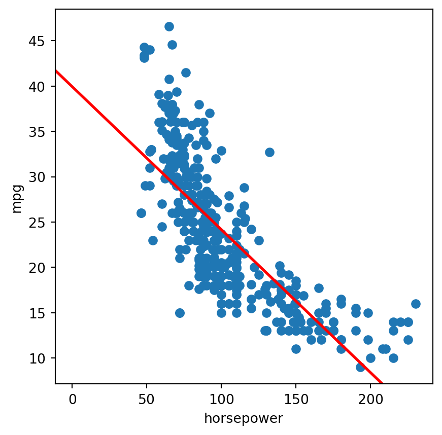
# there is no attribute called name in 'auto' datasetpredictors = auto.columns.drop(['mpg'])X_9 = MS(predictors).fit_transform(auto)model_9 = sm.OLS(y, X_9)results_9 = model_9.fit()summarize(results_9)
Yes, there is a relationship between the predictors and the response.
Even with suspected huge multicollinearity, which tends to hid significant variables, all other predictors excpet cylinders, horsepower, and acceleration appear signidicant to the model.
A one year increase, keeping all other factors constant, is associated with a 0.7508 change in mpg.
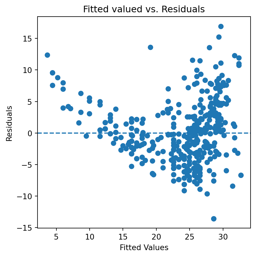
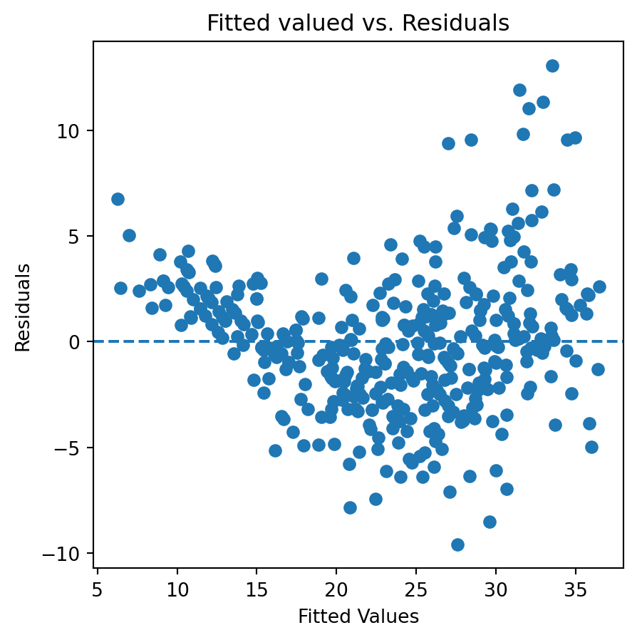
fig, ax = plt.subplots(figsize=(5,5))ax.scatter(results_9.predict(), results_9.resid)ax.axhline(0, linestyle='--')ax.set_title('Fitted valued vs. Residuals')ax.set_ylabel('Residuals')ax.set_xlabel('Fitted Values')plt.show()
The residual vs. fitted plots suggest that, similar to the simple linear regresion we fitted earlier, there is osme non-linearity we haven’t captured yet.
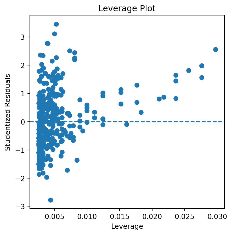
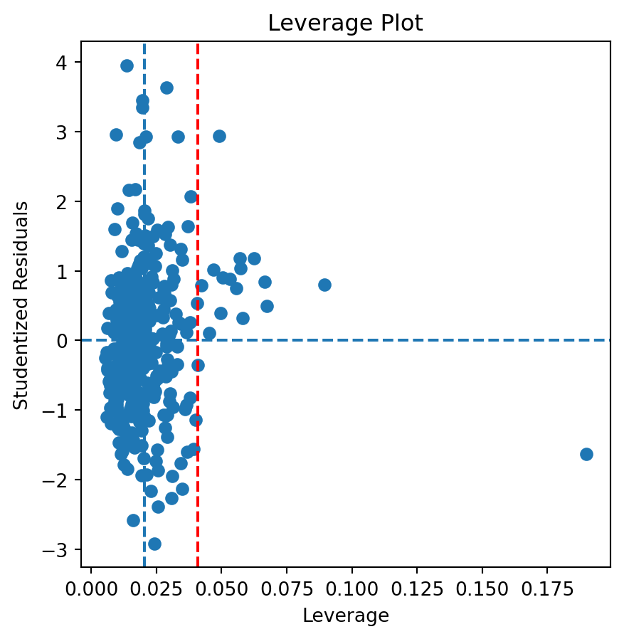
There are some points that both exceed the average leverage and are greater that |2| studentized residuals. There are a few points that exceed similar limits for the studentized residuals while reaching past 2 times the average leverage. One point can be seen with really high leverage but within |2| studentized residuals. Outliers clearly exist, with most being below two times the average leverage. There definetely is an unusual high leverage going on here.